Adaptive Predictive Reinforcement Learning: Entropy-Driven Adaptive Prediction Horizons

PROPOSED MODEL
ONGOING

2024 - Present • Aston University

Table of Contents


1. Overview

Entropy-guided horizons for faster, safer RL

Fixed prediction horizons lead to wasted computation in easy scenes and brittle planning in complex ones. This project uses policy entropy to adapt the depth of world-model rollouts on the fly. Early results show faster convergence in LunarLander-v2 and stronger success/return trade-offs in LiteSocNavGym, while keeping inference latency suitable for robotics.

Time
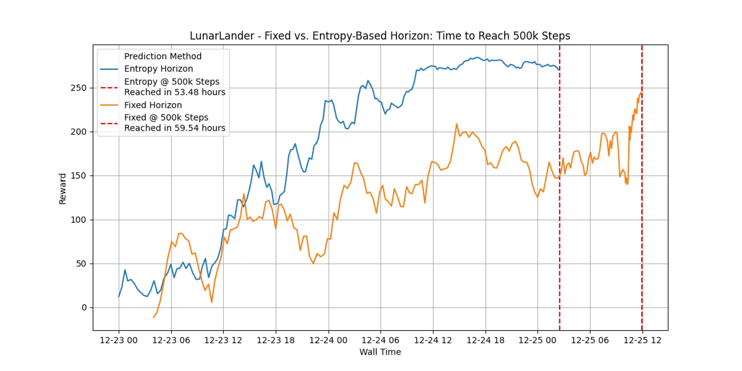
53.48 h to 500k steps
Entropy horizon vs 59.54 h fixed (LunarLander)
100%
Success rate
SAC + CGLSTM (adaptive) in LiteSocNavGym
5.62 days
Full training
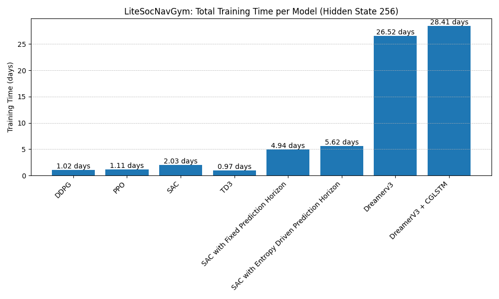
LiteSocNavGym vs 28.41 days for DreamerV3 + CGLSTM
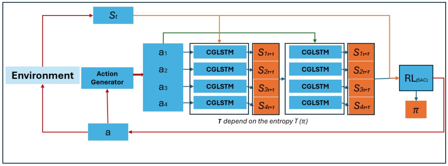
Adaptive prediction horizon pipeline

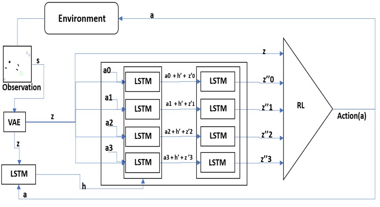
Adaptive horizon pipeline: policy entropy controls how many CGLSTM rollouts are generated before the SAC update.


2. Research Motivation


3. Adaptive Architecture

The adaptive controller sits between the CGLSTM world model and the reinforcement learner. At each step it samples multiple horizon candidates, evaluates expected entropy reduction, and commits to the smallest depth that meets a confidence threshold.

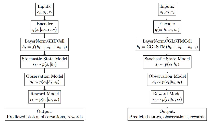
Flow diagram comparing DreamerV3 GRU and DreamerV3 CGLSTM

Replacing the LayerNorm GRU in DreamerV3 with CGLSTM gives higher fidelity latent rollouts before the adaptive controller is applied.

LiteSocNavGym rollout diagram with adaptive prediction horizon

Adaptive horizon inside LiteSocNavGym: when policy entropy spikes, additional CGLSTM rollouts are appended before the SAC update.


4. Implementation Notes

def choose_horizon(entropy, candidates=(1, 2, 4, 6, 8), thresholds=(0.2, 0.35, 0.5, 0.65)):
    horizon = candidates[0]
    for h, t in zip(candidates[1:], thresholds):
        if entropy > t:
            horizon = h
        else:
            break
    return horizon

entropy = policy_entropy(obs)
steps_ahead = choose_horizon(entropy)
rollout = world_model.rollout(obs, steps=steps_ahead)
value, action = sac.update(rollout)

5. LunarLander Experiments (500k steps)

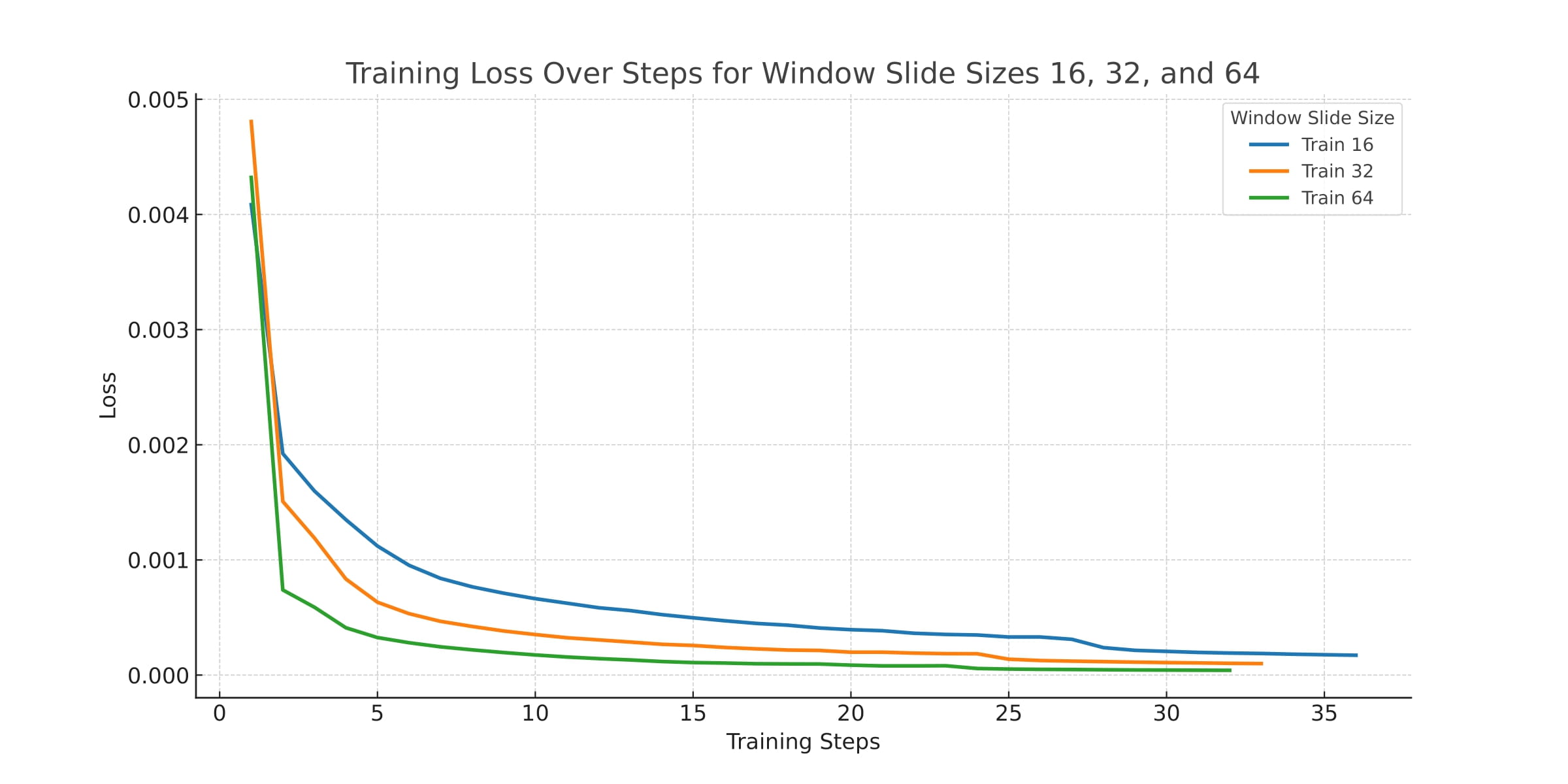
5.1 Window-slide selection for CGLSTM

Training loss over steps for window slides 16, 32, 64

Entropy controller uses a 32-step window (middle curve) – fastest loss decay without the instability seen for 16.

5.2 Horizon candidate comparison

Reward curves comparing two horizon sets

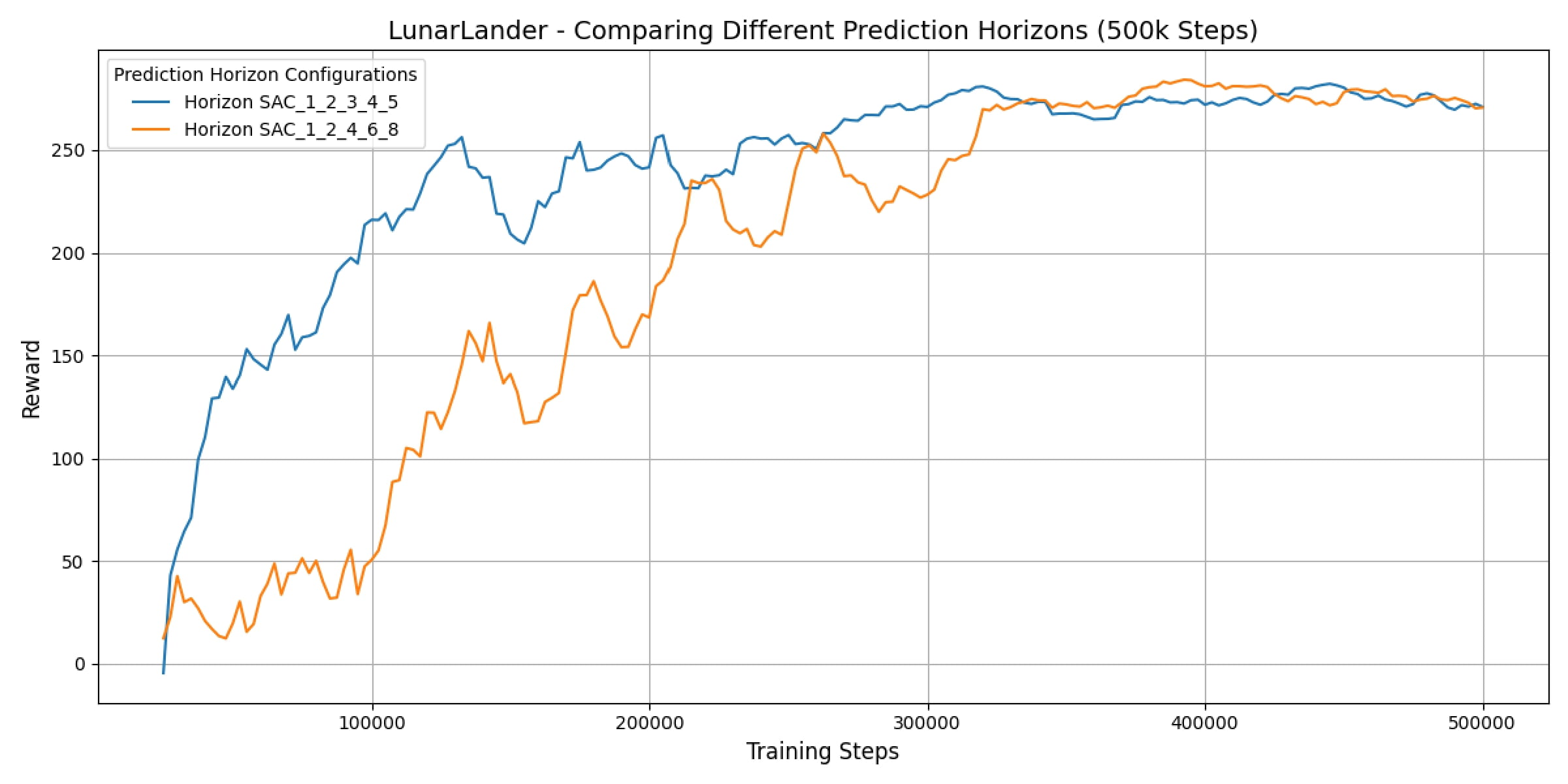
Candidate set {1,2,3,4,5} converges quickly; {1,2,4,6,8} overtakes after 200k steps. Set B selected for final runs.

5.3 Training performance

Training results for LunarLander

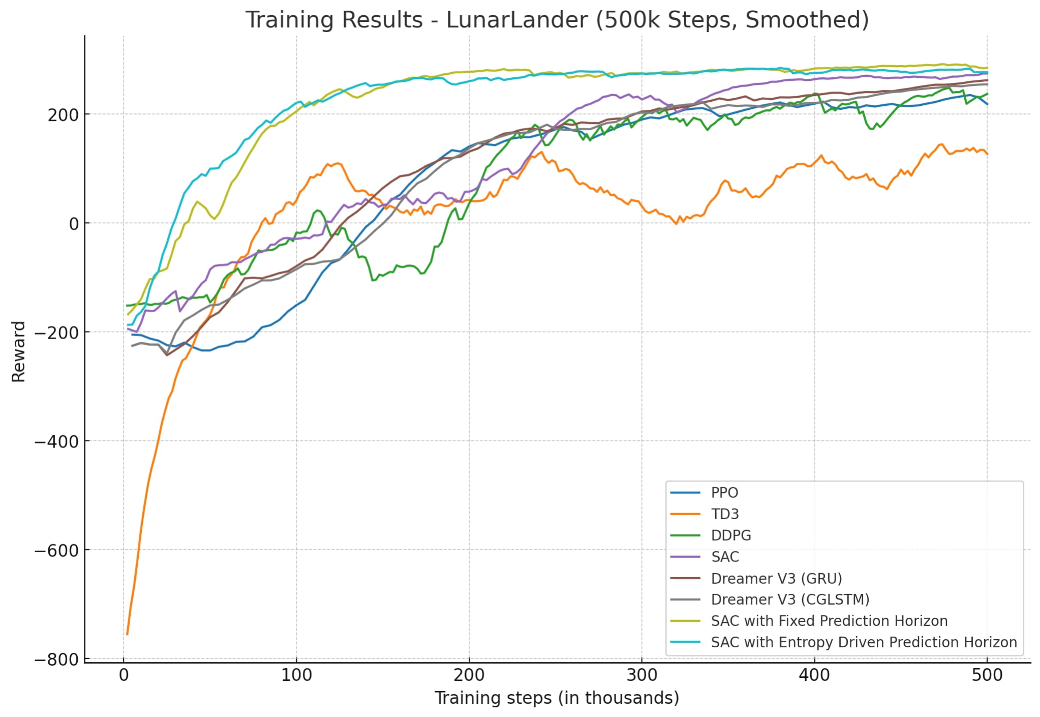
Entropy-driven horizon (cyan) matches DreamerV3 + CGLSTM convergence while remaining stable after 350k steps.

5.4 Wall-time savings

Wall-time comparison fixed vs entropy horizon

Entropy controller reaches 500k steps in 53.48 hours (blue) vs 59.54 hours for the fixed horizon baseline (orange).


6. LiteSocNavGym Experiments (4M steps)

6.1 Training reward progression

Training results for LiteSocNavGym

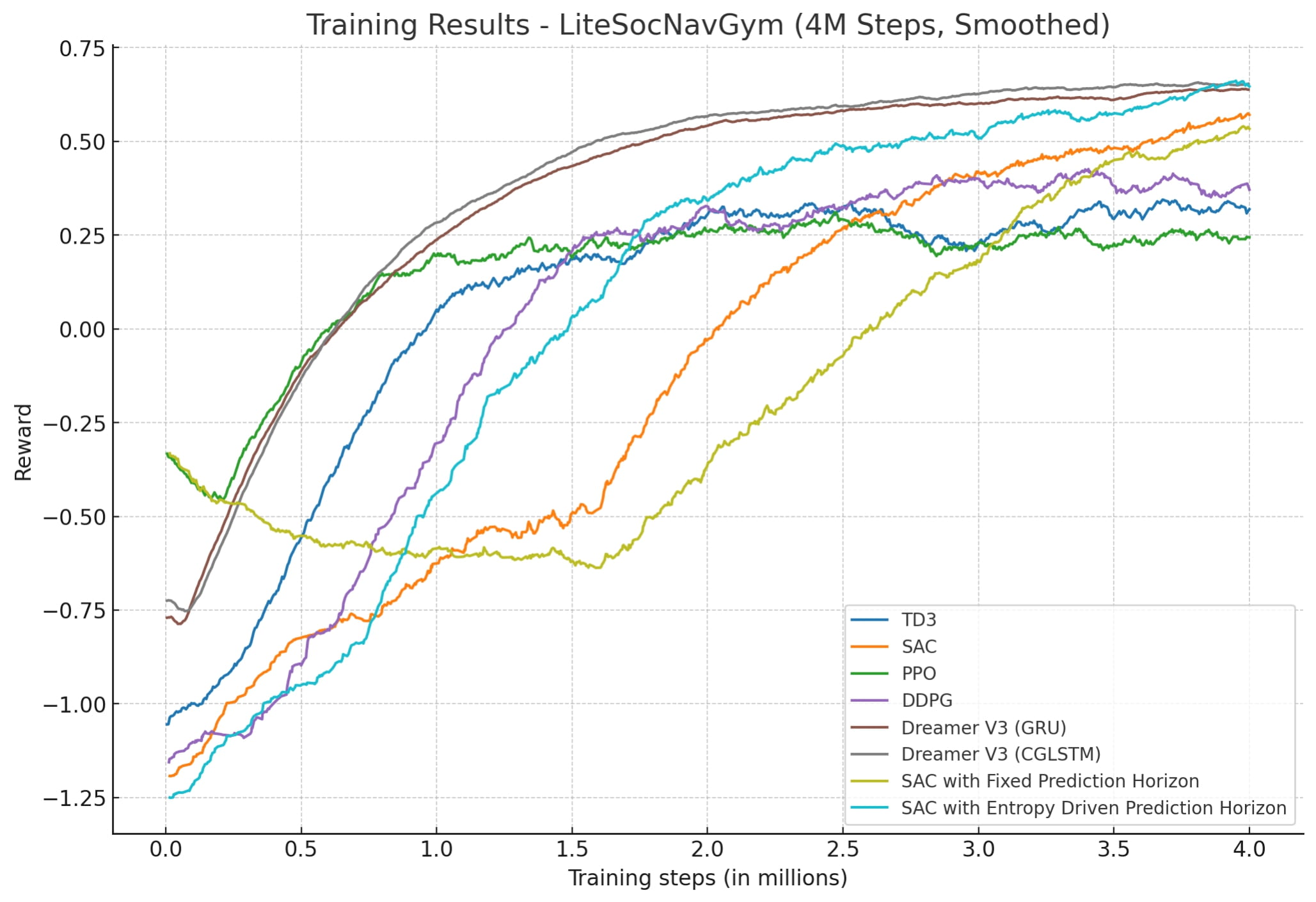
Adaptive horizon (cyan) and DreamerV3 + CGLSTM (brown) are the only agents sustaining positive reward after 3M steps.

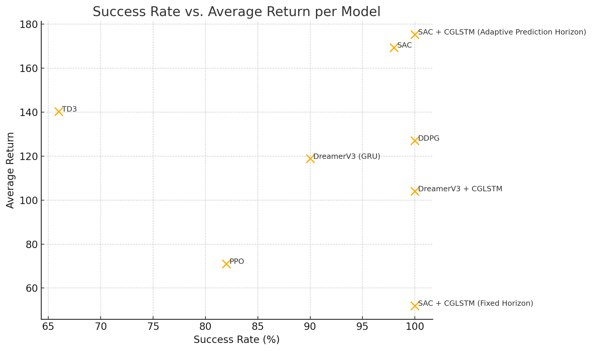
6.2 Success rate vs average return

Success rate vs average return

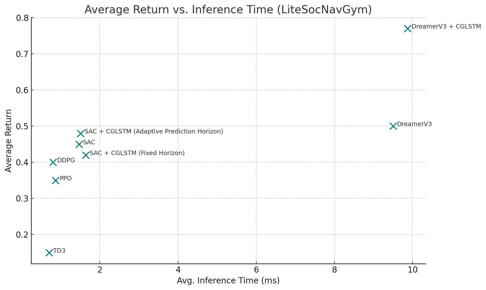
Adaptive horizon with CGLSTM achieves ~0.48 average return at ~1.6 ms inference, outperforming PPO/TD3 in both axes.

6.3 Training cost profile

Training time comparison

Adaptive horizon needs 5.62 days to train (hidden size 256), versus 28.41 days for DreamerV3 + CGLSTM.

6.4 Success vs return scatter (aggregate)

Success vs average return for adaptive variants

Scatter from viva slides: adaptive SAC variants dominate the top-right corner (high success, high return).

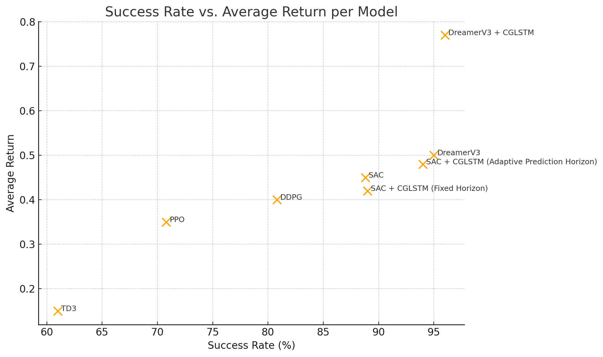
6.5 Dreamer comparison

DreamerV3 and DreamerV3 + CGLSTM comparison

DreamerV3 + CGLSTM (orange marker) obtains the best success/return compromise, justifying its role as a teacher for adaptive SAC.


7. Current Status & Next Steps

Completed so far:

Next steps:


Technologies: Python • PyTorch • Gymnasium • SAC • DreamerV3 • CGLSTM

← Back to Research Portfolio